3.6 Truly 3-dimensional data
Introduction
Some environmental management problems require the storage, handling, analysis and display of all three dimensions, rather than simply the quantification of the shape of the Earth’s surface, as occurs with a DEM. Obvious examples of natural resource management problems requiring truly three-dimensional data lie in oceanography (for example, in documenting ocean temperatures at different depths and consequent implications for spatial distributions of marine wildlife and their ecological management), in geology (whereby the boundaries of strata or faultlines may be defined by x, y, and z coordinates and required for modelling geohazards), and in atmospheric science (for example in modelling pollutant dispersion through the atmosphere and subsequent deposition). Similarly, there is a growing body of literature looking at 3-dimensional data structures for buildings (Figure 1), which again have environmental management applications in for example the planning of urban street trees, green spaces, and domestic renewable energy. It is clear from these examples that a 2.5 dimensional DEM structure is inadequate for handling such features. A borehole, for example, may be defined by a single x, y coordinate pair, yet comprise a series of vertical polyline features, each representing different strata and with different start and end z coordinates. A single z coordinate attached to the point (i.e. a spot height) would be insufficient to record the complexity of the borehole’s subsurface characteristics.
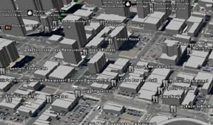
Figure 1: A 3-dimensional model of a city. Courtesy of Google Maps
Data structures for truly 3-dimensional data
Given this broader need for 3-dimensional data, some GIS systems now incorporate data structures that enable handling of such phenomena. One solution to this problem is the voxel or volumetric pixel, essentially a three dimensional extension to the concept of the raster (see references), widely used in computer games as well as for geospatial data. The NetCDF format provides one commonly encountered mechanism for using voxels and is described elsewhere in this module. As an extension of the raster, voxels suffer similar drawbacks, for example in having a fixed spatial resolution that cannot be adapted to represent particularly important geological strata, regions where there is rapid change in atmospheric or geological conditions, or greater data availability. However, there is again an alternative data structure that can be adapted from 2-dimensional GIS to resolve this problem. In much the same way as quadtrees can be used to represent 2-dimensional spatial data using a variable grid resolution, there is a 3-dimensional equivalent of the quadtree, the octree, that also uses a variable grid resolution. Dunstan and Mill (1989) provide a classic introduction to the octree’s use with geospatial data, and algorithms for octrees remain an active research area in 3-dimensional data processing to this day.
In the same way that there are 3-dimensional equivalents to 2-dimensional grid-based data structures such as the raster and the quadtree, so there are 3-dimensional equivalents of vector feature types that go beyond the 2.5 dimensional contour or spot height. Within ArcGIS, examples of such structures include 3-dimensional points, polylines, and polygons, in which vertices describing the boundaries of polygons or paths of polylines have a height value as well as x and y coordinates. ESRI have also developed a data structure known as a multipatch to handle three dimensional features. The multipatch, which comprises different triangles or other surfaces linked together to form 3-dimensional objects, is particularly well suited to the representation of buildings. Textures can be attached to the constituent surfaces that make up a multipatch, enabling more realistic visualisation of buildings. Multipatches can be closed (forming a volume enclosed by a set of surfaces) or open (forming a surface in three dimensional space), though in practice closed multipatches are typically used for buildings are relatively simple geometric forms.
Visualisation of 3-dimensional environmental data
Monitoring an earthquake using 3 or more listening devices (geophones) allows the location of its epicentre (the source of the earthquake) to be fixed. Mapping multiple epicentres can reveal 3 dimensional geological structures such as faults. The latter part of the article by Chesnaux et al (2011) includes some examples of other methods for visualising 3-dimensional data. One such example is the fence diagram or geosection (the latter being the term used within ESRI’s Arc Hydro Groundwater), in which a set of 3-dimensional transects through the subsurface of a study area are used to display the spatial distribution of geological star
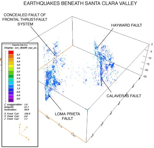
Figure 2: Earthquakes plotted in 3-dimensions in blue. Courtesy of USGS.
Performing analytical operations on 3-dimensional data
Once data structures such as the multi-patch have been developed to describe 3-dimensional phenomena such as aquifers, tree crowns, and buildings, then it follows that analytical operations are required in order to process these features. For example, just as 2-dimensional features can be intersected, to identify the areas common to two sets of polygons, so 3-dimensional features can also be intersected, thereby identifying the volume common to two sets of 3D polygons. Similarly, it would be possible to conceive of a 3-dimensional buffer zone, analogously to a 2-dimensional buffer zone.
Activity
Download this practical exercise and tackle the activity described in the pdf, which involves downloading, visualising and conducting basic analysis on multipatch data representing various geological strata in the Nottingham area of the UK.
References (Essential reading for this learning object indicated by *)
The GIS wiki site provides an introduction to the concept of a ‘voxel’: http://wiki.gis.com/wiki/index.php/Voxel.
Chesnaux, R., Lambert, M., Walter, J., Fillastre, U., Hay, M., Rouleau, A., Daigneault, R., Moisan, A., and Germaneau, D. (2011)vBuilding a geodatabase for mapping hydrogeological features and 3D modeling of groundwater systems: Application to the Saguenay–Lac-St.-Jean region, Canada. Computers and Geosciences 37 (11), 1870-1882.
Dustan, S., and Mill, A. (1989) Spatial indexing of geological models using linear octrees. Computers and Geosciences 15 (8), 1291-1301. http://www.sciencedirect.com/science/article/pii/0098300489900939
ArcGIS groundwater Data Model: http://www.archydrogw.com/Main_Page
Introduction to groundwater: http://pubs.usgs.gov/gip/gw/
The data used in the practical exercise are taken from the British Geological Survey web site here: https://www.bgs.ac.uk/geological-data/datasets/