3.5 Visualisation using elevation
Many actions in environmental management affect the visual appearance of a landscape as well as the natural resources within it. For example, building a visitor centre within a national park introduces a new building into the landscape, whilst carrying out a controlled burn of heath land will leave a visual ‘scar’ on the landscape for several months. It is becoming increasingly important to quantify the visual impact of environmental management options as well as their impact on ecological or water resources. DEMs can be used to help assess these visual impacts. More generally, visual depiction of landscapes, particularly simulated landscapes, can be a powerful way of communicating with the public and engaging them in the environmental decision-making process (Appleton et al, 2002;
Rural areas are increasingly used for recreation and tourism and rural landscapes are said by natural resource economists to have an ‘amenity value’, an inherent value to those who use them. Much recent GIS work (e.g. Scottish Natural Heritage / the Countryside Agency, 2003) has attempted to identify the perceived character of the landscape and 3-dimensional visualisation is related to this process of landscape character assessment.
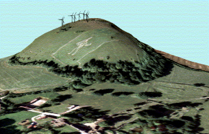
Figure 1: A 3-dimensional view of a fictitious proposed wind farm above Figure 1: A 3-dimensional view of a fictitious proposed wind farm above the Cerne Abbas archeological site in the UK. (Source: the GeoData Institute)
3 dimensional visualisation
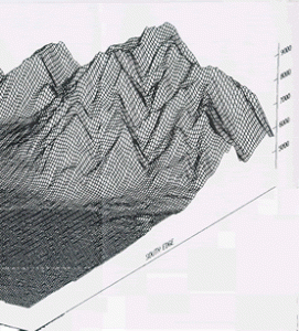
Figure 2: A DEM with shadows and one as a wire frame. Courtesy of USGS
One way of assessing the visual impact of new construction is to produce a 3-dimensional scene indicating what a proposed construction project might look like. Such 3-dimensional views can be used to support planning applications and provide a means of communicating planning proposals to the general public. By using 3-dimensional views, GIS can be used to assess the visual impact of a particular feature before it is actually introduced into the landscape. Such 3-dimensional views have several components:
- A surface image, which is usually a DEM. To make a 3-dimensional landscape view more dramatic, sometimes a vertical exaggeration factor is used, which artificially increases the 3-dimensional display of vertical differences in elevation relative to horizontal distances on the ground.
- A ‘drape’ image is often used to shade the DEM. Sometimes aerial photographs are used as ‘drape’ images. Often, the ‘drape’ image shows the amount of light falling on each grid cell to make the 3-dimensional visualisation more realistic. The amount of light falling on each grid cell can also be calculated from a DEM and is known as analytical hill shading. For more details of this calculation, see the illustrations below. Typically, such calculations assume that the sun is at a fixed point. The sun’s height is specified as an azimuth (i.e., an angle to the horizon) and its relative position as a compass bearing. In some cases, analytical hill shading can be combined with a map layer depicting, say, land cover before being used as a ‘drape’ image. Sometimes, a 3-dimensional display is produced without a ‘drape’ image with only the outlines of each DEM grid cell drawn. This is known as a wire-frame display (see illustration above).
- A viewer perspective, which specifies the location of the viewer relative to the DEM. In some 3-dimensional visualisations, the location of the viewer is static. In other visualisations, the viewer’s location can be changed dynamically, producing a ‘fly-through’ in which the observer can look at the landscape from many different vantage points.
- In more sophisticated 3-dimensional visualisations, atmospheric conditions such as haziness and cloud cover can be specified to make the display even more realistic.
Viewsheds and line-of-sight calculations
Often, it is important to be able to predict the places from which a new building or forestry plantation may be seen. The area that can be seen from a particular point in the landscape has traditionally been referred to as a viewshed. However, more recently the phrase zone of theoretical visibility (ZTV) has been used, particularly in landscape architecture (Foote, 2009). The term ZTV is used particularly in connection with the viewshed output from a ‘bare earth’ DTM rather than a DSM that incorporates object heights because it is a worst case scenario. In reality, the extent of the visual impact may well be less than the ZTV suggests because vegetation, buildings and other objects may obscure landscape features from view. Follow-up fieldwork is often necessary to ascertain whether the ZTV is borne out in reality.
Many GIS packages can calculate the extent of a viewshed for a given target feature (e.g. a series of pylons or a new building) from a DEM. This type of operation is known as an inter-visibility calculation. Other forms of inter-visibility calculation also exist. For example, a line-of-sight calculation identifies those sections that are visible along a line drawn from an object to viewer and can be thought of as the linear equivalent of the areal viewshed calculation. Heuvelink (1998) classifies GIS operations as being cell-based (where calculations are based on individual grid cells only), local (where calculations are based on each cell and its immediate neighbours) and global (where calculations are based on distant grid cells as well as immediate neighbours). According to this classification, inter-visibility calculations can be described as a global GIS operation.
The accuracy of an output viewshed map layer depends on the grid resolution, data source and interpolation method of the DEM from which it was derived. However, Heuvelink (1998) suggests that it is difficult to quantify the accuracy of the output raster grid produced using such global operations, even if the accuracy of the input DEM is already known. One method of assessing a viewshed’s accuracy is to make observations about the inter-visibility of landscape features in the field and compare these to the viewshed predicted from a DEM. Where the accuracy of the input DEM is known, an alternative approach is to generate a random error term, add this to the DEM and see what effect this has on the calculated viewshed. By generating random errors many times and calculating viewsheds, it is possible to assess the accuracy of the output viewshed map layer. This approach to assessing the accuracy of a viewshed is known as a Monte Carlo simulation.
Activity
3 dimensional visualisation using GIS
If you are using ArcGIS Desktop, download the attached zip file and undertake the GIS exercise included in the pdf file. This involves creating a 3-dimensional fly-through a DEM for a forested area. If you are using ArcGIS Pro, download this zip file and undertake the exercise, which will introduce you to 3-dimensional fly-through’s via the software’s scene functionality.
References (Essential reading for this learning object indicated by *)
This article provides a brief description of inter-visibility calculations from a practical, landscape design perspective:
Foote, R. (2009) Landscape Portrait. Renewable Energy Focus 10 (4), 30-31.
For an example of DEMs being used for 3-dimensional visualisation, see: http://www.satimagingcorp.com/services/3dterrain/
This article discusses the issues involved in visualising landscapes using GIS:
Appleton, K., Lovett, A., Sunnenberg, G., and Rocketry, T. (2002) Rural landscape visualisation from GIS databases: a comparison of approaches, options, and problems. Computers, Environment and Urban Systems 26 (2-3), 141-162. http://www.sciencedirect.com/science/article/pii/S0198971501000412
Although not directly related to visualisation using DEMs, it is worth being aware of the related concept of landscape character assessment. You can find out more about this on Natural England’s web site: http://www.naturalengland.org.uk/ourwork/landscape/englands/character/default.aspx
The following book is the origin of the concepts of cell-based, local and global operations described above. Note that you are not intended to read it and it is cited here as a reference only:
Heuvelink, G. (1998) Error Propagation in Environmental Modeling with GIS. Taylor and Francis.