3.1 Into the third dimension – digital elevation models

The attribute elevation is typically expressed relative to a vertical datum, which typically either relates to sea level or to a local geodetic surface or geoid. A geoid is a form of three-dimensional surface of equal gravitational potential and such surfaces take into account local gravity variations across the Earth’s surface. Geoids also underpin the horizontal datums that are used with geographic coordinate systems, such as World Geodetic Survey 1984 (WGS 1984). With sea level, elevation is often expressed relative to mean sea level, in other words, a long-term average sea level from which the effects of tides, weather conditions and so forth have been averaged out. Mean sea level is affected by local variations in gravity, so its exact meaning varies locally. In the UK, elevation is expressed relative to a local Ordnance datum, which is based on a long-term set of sea-level measurements at Newlyn, Cornwall from 1915-21. An older vertical datum, based on sea level measurements taken at Liverpool, is also occasionally used in the UK. An elevation of 0 metres AOD (Above Ordnance Datum) indicates an elevation that corresponds to mean sea level, whilst positive values are above mean sea level and negative values below mean sea level.

As digital representations of relief, DEMs are approximations of a continuous surface. The method of approximation will vary depending on the source data available to create the DEM, and the intended use of the DEM. The three main forms of DEM are illustrated below; as you look through them, think about the most appropriate uses for each, and their relative strengths and weaknesses when used in a GIS.

Contours and spot heights

Contours are widely used in paper maps because they allow height information at a known precision to be easily measured and used. When represented digitally, contours are a vector based GIS technique, being represented by polylines following the land surface at specified height values, or regions of a specified height interval, bounded by the contour polylines.

The line node frequency (the number of different x and y co-ordinate pairs within a given length of contour) determines the level of surface detail that is captured by a contour. As the node frequency is normally variable, this provides an efficient method of representing the surface, node frequency increasing with the surface complexity. This keeps the data volume to a minimum.

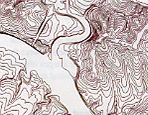
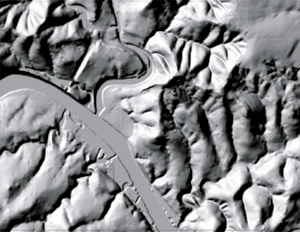Figure 1: A landscape on the left as a contour plot on the right. Courtesy of USGS.

The threshold for the representation of surface detail is the vertical interval between contours. By convention this is a fixed value for a data set, and is a trade off between unnecessarily many contours on steep slopes and too few in flatter areas.

Contours do not explicitly record inflections in the surface detail such as ridges, gully lines, or breaks in slope, which are important for geomorphological analysis. In sloping regions, ridges and gullies can be inferred from the inflection points of successive contours, but this technique breaks down in flatter areas, and additional topographic information may be needed.

Triangulated Irregular Networks (TINs)

Triangulated Irregular Networks are another way of approximating a surface. The surface is represented by flat triangles of varying shape that are connected along their edges to approximate relief. The concept is best illustrated through a diagram: see the illustration at the following web address in the references.

The ‘irregularity’ of a TIN allows the density of points to vary with the complexity of the surface being modeled, making it a very efficient format in data storage terms. In areas of low relief the points can be widely spaced, giving larger facets, and as the surface becomes more complex, the point density can be increased until features are represented with the accuracy required. However, they differ from contours in that they are better at defining a change in slope.

Contours are a set distance apart so it can be difficult to distinguish where a change in slope occurs. In the diagram below a contour map of a slope is shown where slope changes. With contours the location of the change of slope is not well defined, and so both cross sections produced from the contours are valid. One has the change of slope at the same point as a contour, whilst another has the break up the slope from that contour.

Figure 2: Illustrating how contours may or may not appear at breaks of slope

The way a TIN is calculated means it will probably have the boundary of 2 of the triangles at the break of slope. This can be useful when the terrain has breaks of slope that are important to map such as erosion gullies in an area of otherwise low relief.

Triangulation is the process by which the spot heights are interconnected. The most commonly used method of achieving this is called the Delaunay Triangulation. Delaunay Triangulation is built to fulfil the condition that the circle that passes through the three vertices of each triangle (the circumcircle) does not enclose any other triangle. Triangulation produces a surface of facets within the convex hull of the input data points (see the references below for further details of this process).

Figure 3: Delaunay Triangulation

Figure 3 shows Delaunay Triangulation, nodes are shown as black dots, and the connecting lines as black lines. The three coloured triangles each have their circumcircle shown in their corresponding colour. Note that none of the circumcircles completely encloses another triangle.

Although irregular in nature, the triangular basis of TINs means that they can be analysed using simple geometric techniques, though these may not be standard tools in a desktop GIS. Visually a TIN can appear angular and artificial, but as triangulation is widely used as the basis for three dimensional computer graphics, many techniques exist for making their appearance more realistic, such as Gouraud shading.

Continuous Grids

Continuous grids are DEMs that store a height value for each cell in a regularly spaced grid or matrix, and are a raster based approach to representing a surface. Figure 4 shows a large scale view of a continuous grid shows the individual cells, coloured by their height value:

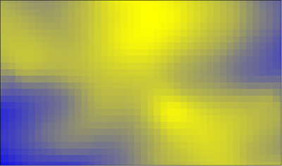
Figure 4: A continuous grid of shades with height represented as a shade between blue and yellow

The regular spacing of a continuous grid has a number of implications for the data format. The grid cell size determines the smallest feature that will be represented on it, but the same cell size has to be applied over the extent of the grid. If the surface being modeled varies in complexity then a continuous grid format will store unnecessary quantities of data in the flatter areas, increasing the storage space and processing time required for the data set. Continuous grids are rectangular in extent, with cells outside the area of interest being ignored, or set to a null value, but still contributing to the data volume, and whilst large grid files can be compressed using conventional lossless raster techniques, this will not improve the time taken to process them.

Regular, pre-specified cell positions mean that ridge lines, gullies and breaks in slope can only be represented by height differences between adjacent cells. This has the effect of making the feature appear more rounded and its position less precise.

In a matrix format, continuous grid data is easily accessed and processed by a computer. Grids of the same cell spacing and extent can be added or subtracted to create new grids. The regular structure allows operations to be carried out on each cell in turn like calculating attributes such as slope and aspect, and performing general image processing operations such as filtering and smoothing.

Out of the three formats discussed above, the most widely used is the Continuous Grid, the falling prices of data storage capacity and processing power making the disadvantages of the format less significant. ‘Continuous Grid’ is now commonly seen as being synonymous with the term ‘DEM’, and many applications exist to create derive DEMs in contour and TIN formats from continuous grid data.