Filtering and DTM Generation
This learning object explains the application of different filtering techniques in order to derive a digital elevation model (DEM) from Airborne LiDAR data.
Before we proceed, we need to revise our understanding of different products that can be generated from Airborne LiDAR data:
Digital Elevation Model (DEM)
There are many definition of a digital elevation model, however we will use the one define by the United State Geological Survey (USGS): “A Digital Elevation Model (DEM) is a digital cartographic/geographic raster data set of elevations in xyz co-ordinates. The terrain elevations for ground positions are sampled at regularly spaced horizontal intervals and void of vegetation and manmade structure”.
Digital Terrain Model (DTM)
The term DEM is often used interchangeably with Digital Terrain Model (DTM). However, strictly speaking, a digital terrain model (DTM) data structure is also made up of x, y points with z-values representing elevations, but unlike the DEM, these may be irregularly or randomly spaced mass points. Direct observations of elevation at a particular location can be incorporated without interpolation, and the density of points can be adjusted so as best to characterize the actual terrain. Fewer points can be used to describe very flat or evenly sloping ground; while more points can be captured to describe very complicated terrain.
Digital Surface Model (DSM)
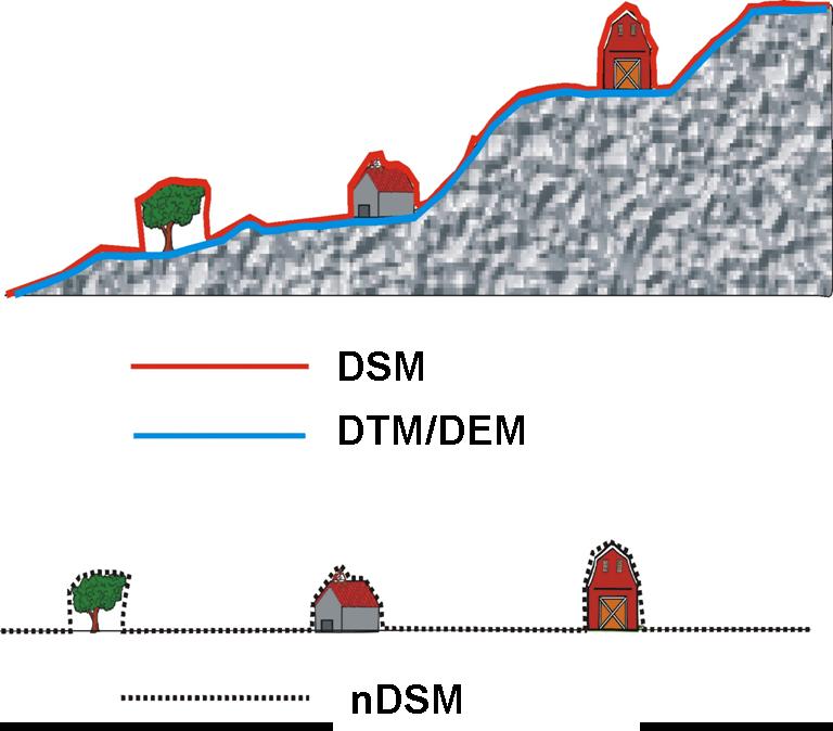
A digital surface model (DSM) includes features above the ground, such as buildings and vegetation, and is used to distinguish a bare-earth elevation model from a non-bare-earth elevation model. In forested areas this is also referred as Digital Canopy model (DCM). The DSM or DCM is often created form the first return signal of the discrete LiDAR data. The DSM is equivalent to a DTM in open areas and runs on top of vegetation canopies in forested areas and buildings in urban areas.
Normalised Digital Surface Model (nDSM)
The difference between DSM and DTM is called the Normalised Digital Surface Model (nDSM). This helps to reduce the underlying height difference between each object and object heights are represented relative to a plane.
nDSM = DSM-DTM
In order to derive the surfaces mentioned above we need to classify the point clouds into ground points and off terrain points (sometimes with separation of buildings and trees). This is generally achieved by ‘filtering’. Once we have the ground points then we can make the DEM and DSM by interpolating the points into a specific grid. Gridded DEMs are much more efficient to display in GIS software. Pixel size is an important parameter while producing gridded products: if the pixel size is large then we lose lot of detail in interpolation. On the other hand, if we choose a smaller pixel size we have fine detail but this will result in large files. However, in any case the pixel size of the grid should never be smaller than the nominal point spacing of the raw LiDAR point cloud.
A number of algorithms have been proposed to filter the point cloud and then generate the DEM or DSM. We will cover some of the commonly used ones here: They are:
- Block minimum filters
- Morphological filters
- Surface based filtering
- Segmentation based filters
Block minimum filters
These are simple filters which takes the minimum elevation within a certain block (area). If the area is a raster grid then it finds the lowest point within that grid cell and assigns that directly to the elevation of that grid cell. However, the performance of this algorithm depends on the grid size and position. In addition, there is an inherent assumption of flat terrain and the algorithm does not perform well in inclined terrain.
Morphological filters
Morphology in remote sensing is based on two fundamental operations: dilation and erosion. Dilation or the opening operation is used to enlarge a specific feature, whereas erosion or the closing operation is used to reduce the size of a specific feature. These concepts can be used in LiDAR data, where the erosion operation will retain the minimum elevation within a neighbourhood or window size and the dilation operation will retain the maximum point in the neighbourhood. In general the combination of erosion and dilation are use to filter LiDAR data.
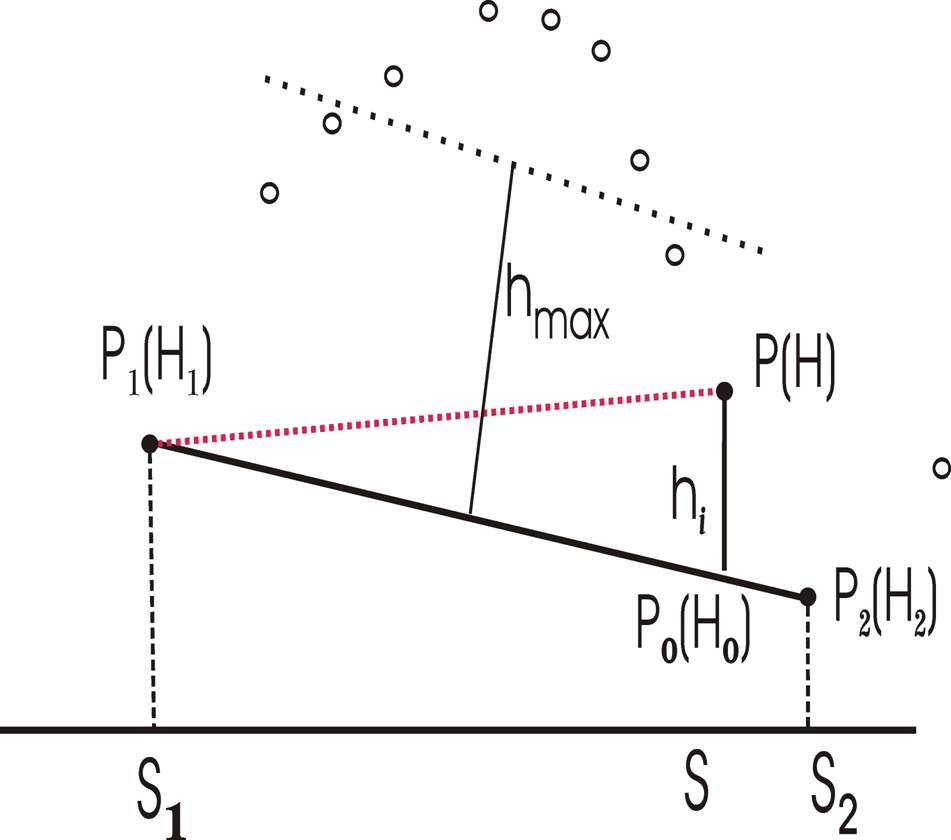
Surface based filtering
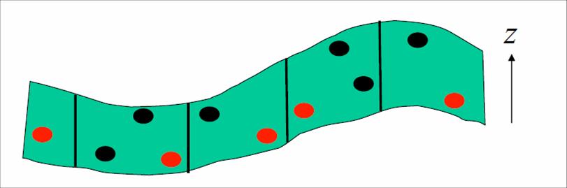
One of the surface based filtering options is the convex/concave hull algorithm. This algorithm first searches for the end and beginning of a convex or concave hull in a 1 dimensional neighborhood and defines a line that connects these points. Then it calculates the distance of the points (hi) which are above/below this line depending upon the convexity or concavity of the hull so that
Min(hi) < hmax
Where hi can be determined by the formula as given below
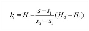
And hmax can be found by the formula
hmax = c*(s2 – s1)
where c is a constant dependent upon the nature of the convex or concave hull.
Then from all the values of hi the smallest one is chosen and considered as a ground point. The algorithm will continue searching for the ground point using the same process it does not find any terrain point.
Segmentation based filters
The process of segmentation groups LiDAR points into height classes or segments. Most segmentation algorithms requires two threshold values: the first one is the minimum height above which points will be classified as off terrain points and the second threshold is the maximum height difference between two neighbouring points to be considered in the same segment.
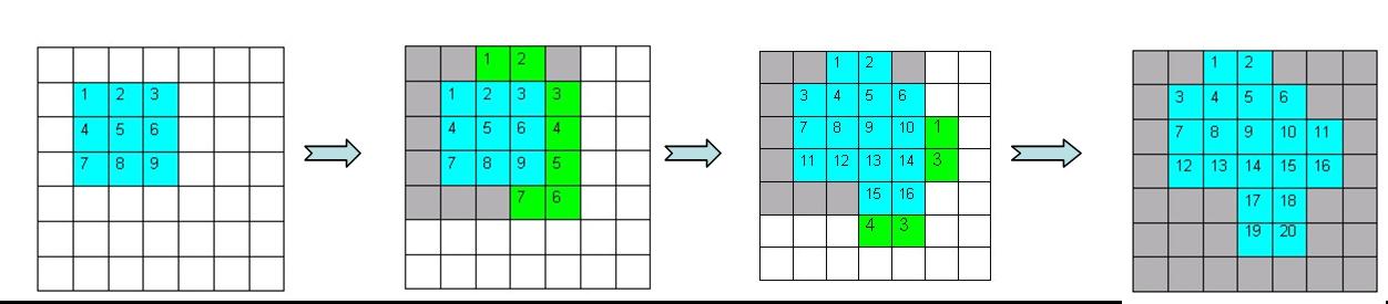
This technique starts by finding some predefined seed pixel (e.g. 3×3) which meets the first threshold requirement and then finding the height difference of all the adjoining pixels. All these pixels whose height difference is below the second threshold are classified as one segment and the process continues until none of the adjoining pixels are below the second threshold.
The figure below provides an example of the segmentation process. In this case, the segmentation process starts when the algorithm found the 3×3 pixels, which are greater than the first threshold (marked in blue). Then it searched for the adjacent pixels in which the height jump is less than the second threshold. Out of 16 adjacent pixels it found only 7 pixels where the height jump was below the second threshold (marked in green). At the end of this process when 16 pixels are included in the segment, the process is repeated again for adjoining pixels and continues until no adjoining pixels are within the second threshold.