8.2. Geometric Correction

The objectives of these materials are:

• to understand the circumstances under which geometric correction is necessary
• to understand different techniques for geometric correction and their strengths and limitations

Geometric correction (sometimes abbreviated to geocorrection) is the process of transforming the X and Y dimensions of a remotely sensed image, so that spatial distortions in the original image are eliminated or minimised and the output X and Y dimensions correspond to a chosen geographic reference system. Examples of geographic reference systems include latitude and longitude, the Universal Transverse Mercator system of projections, and the British Ordnance Survey National Grid. Geometric correction is undertaken to:

1. mosaic together two or more remotely sensed images into a single, combined image
2. compare two or more remotely sensed images of the same area from different times
3. locate points and features of interest on the geometrically corrected image
4. combine a remotely sensed image with data from other sources, such as map layers of national parks or population census data within a GIS
5. accurately calculate distance and area from the geocorrected image

In particular, geometric correction is necessary because satellite flight paths typically do not align with true north and the grid orientation of most geographic reference systems (see figure below).

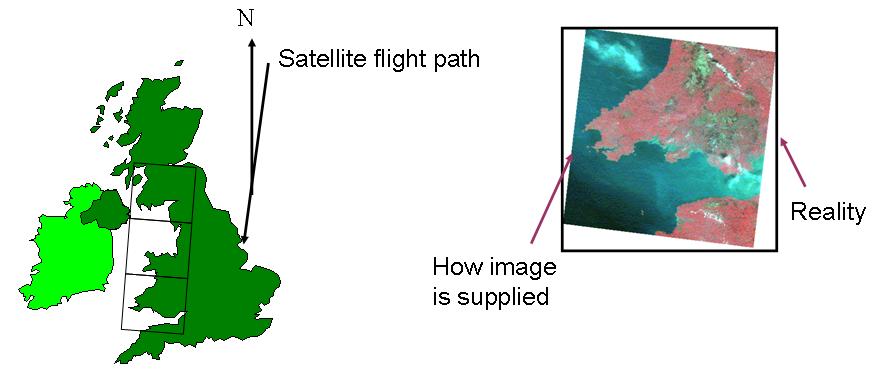
Often, satellite imagery is supplied in a format where geometric correction has already taken place. However, sometimes satellite imagery is provided without any geometric correction having taken place. In either case, it is useful to understand how geometric correction takes place.

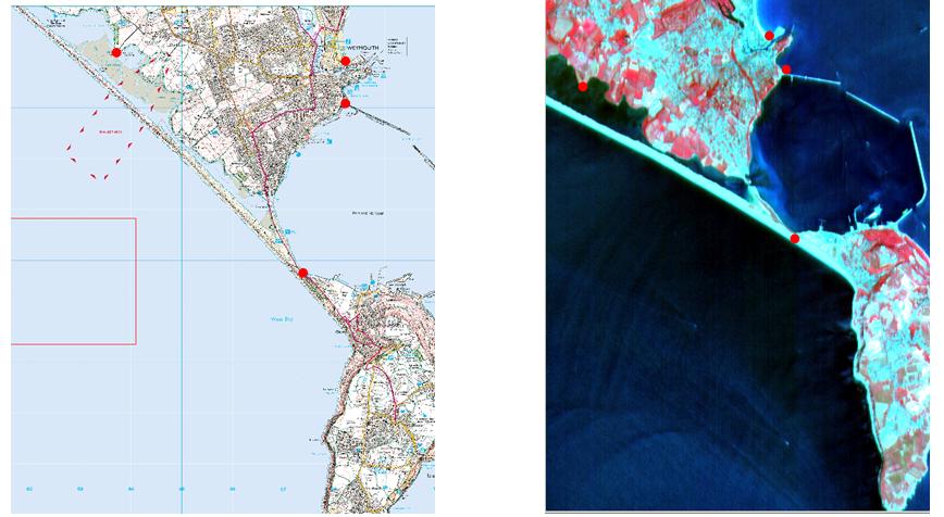
One way of undertaking geometric correction is to use ground control points (GCPs). These points are locations that can be precisely identified both on the remotely sensed imagery and in the target geographic reference system. The coordinates of ground control points in the target reference system can be obtained either by carrying out a Global Positioning Systems (GPS) survey on the ground, or alternatively by identifying GCP locations on a second image or digital map layer that has already been georeferenced. The illustration below shows GCPs (shown as red dots) on a SPOT satellite image that can also be identified on a digital topographic map of the same area. Target reference system coordinates for each GCP can be derived from the digital topographic map and used for geometric correction of the SPOT image.

Ideally, at least 20 ground control points should be collected to geocorrect an image (more points are necessary for some more complex correction procedures) and these points should be well distributed across the image.

Activity

Look at the two images below, showing the locations of ground control points represented as crosses across a  remotely sensed image.

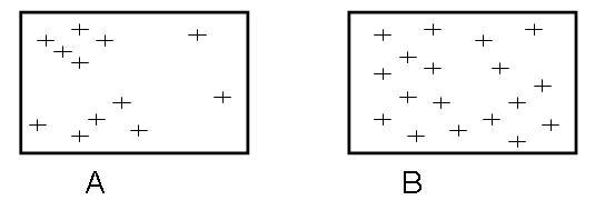
Which of these two sets of ground control points (A or B) would be most suitable for undertaking geometric correction of the image?

Show Answer

Once we have chosen a set of ground control points, we should be able to record their X and Y coordinates in the target geographic reference system (either from ground-based GPS measurements or from existing georeferenced map layers or digital images). We should also be able to record each GCP’s X and Y coordinates in the uncorrected satellite image as column and row positions within the image. These two sets of coordinates for the ground control points (i.e those for the uncorrected image and those for the output reference system or map) can then be used to fit two equations, which transform input X and Y coordinates to the desired output reference system:

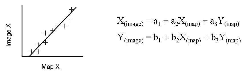
The ‘goodness of fit’ of these equations is often assessed using a measure called the Root Mean Square error (RMS) statistic. The RMS error statistic is typically measured in output map units (e.g. metres in a Universal Transverse Mercator or British National Grid projection). Small values for RMS error are indicative of a successful geometric correction transformation, whilst large values suggest a poorer fit of the transformation. A poor fit may arise either because of problems in locating the GCPs, or because of more complex underlying spatial distortions in the satellite imagery that are not accounted for in the geometric correction process.

The result of geocorrection is to produce a new output grid with its rows and columns aligned with the X and Y (eastings and northings) of a target geographic reference system. However, we still need to take the original values for each pixel in the input image and use these to compute new values for the output grid, as shown below. This process is known as resampling.

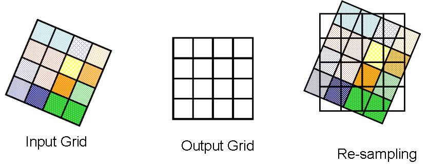
Three different resampling methods are commonly used to calculate output pixel DN values from input DN values:

• nearest neighbour: this method uses the value of the closest pixel in the input image as the new value for the output pixel. The method is thus based on a single input pixel, is computationally fast, and retains the original pixel values. However, it can also lead to some input pixel values being lost and others being duplicated.
• bilinear interpolation: this method uses the weighted average of the nearest four input pixels to each output pixel. The averaging process alters the original pixel values and creates entirely new digital values in the output image. The input pixels that are closest to the centre of the output pixels are given more weight in calculating the average, whilst those that are further away are given less weight. The method tends to be more spatially accurate than the nearest neighbour method and the output image has a less blocky, smoother appearance.
• cubic convolution: this method uses the weighted average of the nearest 16 input pixels to each output pixel. The mean and variance of the distribution of output pixel values match those of the input pixel values, but the data values may be altered. This technique can be used both to smooth an input image and to sharpen it (draw out contrasts). It is the most computationally intensive of the three techniques.

The calculation of output DN values using these three methods is illustrated in the animation below.

N/B: The animation below will not show on the webpage, but you can save/keep them on your computer and view them using the Adobe Flash Player 32 you downloaded earlier