Recent Comments
Archives
Categories
- No categories
Meta
10.1 What is Classification?
Objectives
The aim of this learning object is for students to understand the process whereby data in a remotely sensed image can be used to produce thematic maps and/or tables which show the location and extent of various different land cover types or earth surface features. It introduces the concept of feature space which is essential to an understanding of how image classification works.
Image classification can be thought of as the conversion of ‘data’ to ‘information. In this discussion we will be focusing primarily on the spectral information, which can help us to classify different land cover types (information) from multispectral image data.
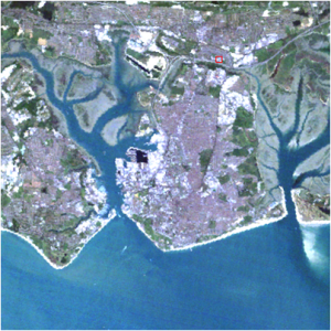
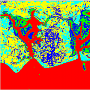
Raw image data and classified land cover information, Portsmouth.
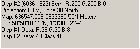
Image classification involves grouping pixels which have similar values. In the following example, we focus on one pixel near the centre of the image. When the data behind the image are inspected, its DN value is found to be 85. Grouping pixels with similar DN values, it is apparent that there are several classes of similar values, which are fairly clearly separated. In this case, our value of 85 is grouped with surrounding similar values in class 5 which encompasses DN values from 44 to 105. This is the class to which it is assigned in the classified image. Generally, the tendency of different pixels of the same land cover type to have similiar reflectance characteristics and hence DN values means that these classes are related to land cover type.

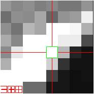
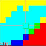
(a) NIR scene with pixel higlighted; (b) detail around central pixel; (c) same area classified
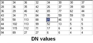

These grids show the treatment of the central pixel highlighted in the images above: the DN value of 85 is assigned, with other similar-valued pixels, to class 5.
In this first example, account has only been taken of DN values from a single (NIR) band. In practice, it is much more powerful to use multiple bands in order to address the question of which pixels have “similar” values and therefore which belong together in the same classes. Examining the clustering of DN values across multiple bands greatly improves our ability to distinguish pixels belonging to different land cover types. Here, we see a scatterplot of DN values of landcover types A and B in the Red and NIR bands.
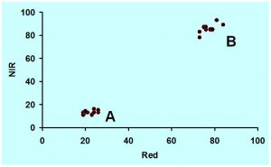
In this example it is clear that land cover types A and B are readily distinguishable by plotting DN in Red and NIR. It is the measurement of distance, or closeness, between pairs of points which allows us to assign each individual value to A or B. In this simple example, the distribution is represented by two axes perpendicular to each other defining a two-dimensional feature space. If we were to introduce a third dimension (e.g. the Blue band), we would have a three-dimensional feature space. More than three dimensions can be considered in just the same way but are difficult to represent visually.
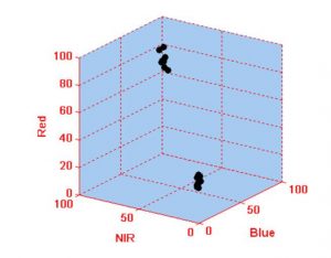
In both the 2D and 3D cases illustrated here, the presence of two clusters of points are recognised by two regions of feature space that have relatively dense distribution of points. Any unknown point might be considered to be a part of cluster A if it is closer to the centre of cluster A than the centre of cluster B. If appropriately defined, these clusters may represent land cover types. The allocation of new pixels to cover types therefore depends on a means of measuring the distance between points in this multidimensional feature space: in the following figure, should pixel C be grouped with cluster A or cluster B?
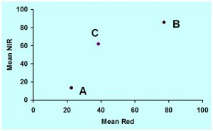
| Red | NIR | |
| A | 23 | 13 |
| B | 77 | 85 |
| C | 40 | 60 |
If the distance between A and C is less than the distance between B and C, then C should be grouped with cluster A. Various different methods have been proposed for finding this distance. The simplest of these is the Euclidean Distance (calculated using Pythagoras’ theorem that you may recall from school maths lessons!)
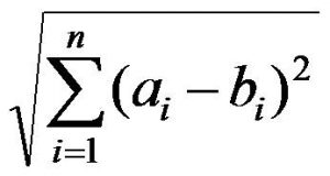
where i is one of the n spectral bands and a and b are pixel values
In the example from the figure above n = 2 (Red and NIR), so the distance can be calculated:
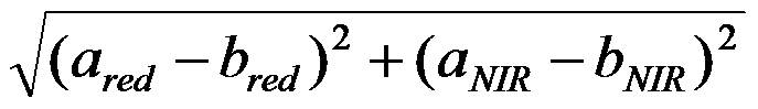
Substituting the values from the example:


BC is smaller than AC, therefore pixel C should be grouped with cluster B.
In practice, digital classification is used in preference to visual interpretation, because
- It is a cost efficient approach to the analysis of large data sets
- The results can be reproduced
- It is more objective than a visual interpretation
- It provides effective analysis of complex multi-band (spectral) interrelationships
Reading Activity
Before proceeding, students should secure their understanding of the basic principles of image classification, and in particular the concept of multidimensional feature space, by reading the relevant chapter in one of the key textbooks:
Campbell, J. B. and Wynne R.H. (2011) Introduction to remote sensing Fifth edition, Guilford Press, London.
(Chapter 12 “Image classification” relates strongly to this learning object)
Mather, P.M. and Koch M(2011) Computer Processing of Remotely Sensed Images Fourth edition, Wiley, Chichester.
(Here, image classification is covered in Chapter 8)