Dan Joyce, our trench supervisor for the 2013 summer field season last year, has written a blog post to summarise his major dissertation project.

Dan studied the University of Southampton Masters in Archaeological Computing last year, which he completed at the end of 2013 (well done Dan from the Basing House team!!!)!

Dan’s project looked at how archaeologists can mesh together different types of archaeological data. Dan is a graduate of the University of Southampton’s Masters in Archaeological Computing run by the Archaeological Computing Research Group.

The course has two major strands to it, one concentrates more on 3D graphics and the theory of archaeological visualisation (Gareth and I are also graduates from this programme), and the other on geographical information systems and survey.

Thanks to Dan for writing this post.

–

CLICK ON AN IMAGE IN THIS ARTICLE TO SEE IT UP CLOSE.

–

Dissertation on the integration of digital archaeological data

Introduction

My dissertation for my masters in Archaeological Computing (Virtual pasts) at the University of Southampton was concerned with integrating different types of digital archaeological data from Basing House. This included a total station and GPS (Global positioning system) topographical survey of the site, a total station building survey of the 16^th century manorial barn, lidar data of the site, geophysical survey data, total station and photogrammetry data and section drawings of the 2013 excavations as well as digital context information.

Topographical and building survey integration

As part of the practical aspect of the Advanced Archaeological Survey course undertaken at the University of Southampton a topographical survey was undertaken on the site using a total station and GPS to record points on the ground. These points were then processed in both the GIS (Geographic information system) software ArcMap and AutoCAD Civil to form a coherent surface. In the case of AutoCAD Civil a TIN (Triangulated Irregular Network) was created, this forms a surface by joining the points together to form triangles (figure 2). In ArcMap a raster DEM (Digital Elevation Model) was created, this forms a much smoother surface by interpolating the surface between the known points (figure 3).

A standing building survey was also undertaken on the 16^th century manorial barn using a total station (figure 1).

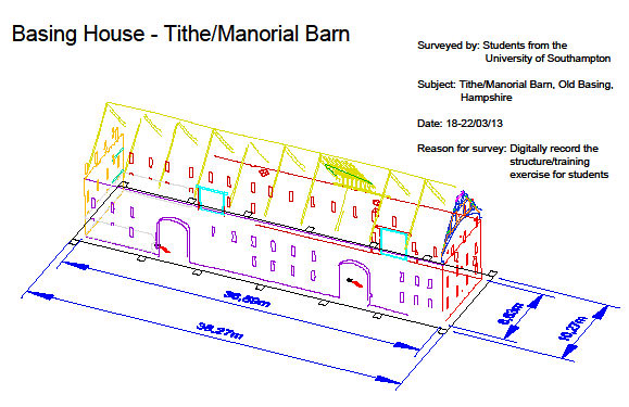
Figure 1 – Total station building survey of manorial barn

The two surveys were combined, with the topographical survey and the building survey appearing together in their correct positions within the British National Grid reference system, as can be seen in figures 2 and 3.

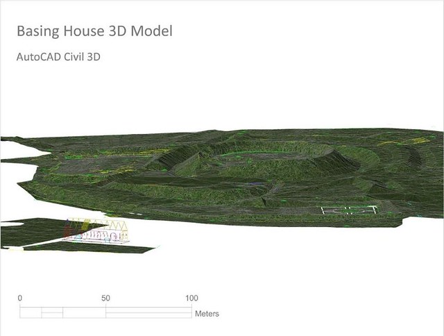
Figure 2 – TIN of topographical survey with the building survey of manorial barn

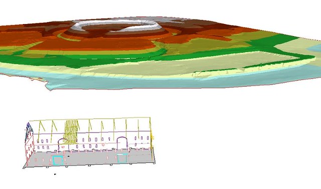
Figure 3 – Raster of topographical survey with the building survey of manorial barn

Geophysical survey integration

As part of the practical aspect of the Archaeological Geophysics course at the university, a geophysical survey of much of the site was undertaken, this involved resistivity, magnetometry and ground penetrating radar surveys. The results from these surveys were integrated with that from the topographical survey within ArcMap as can be seen in figures 4 and 5.

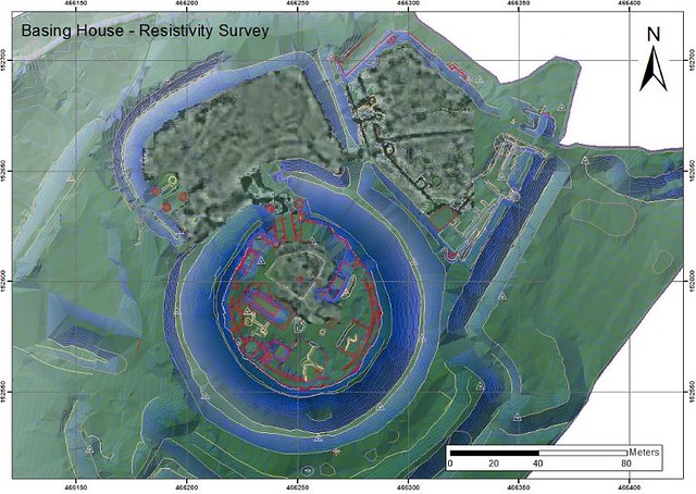
Figure 4 – Resistivity survey overlain on top of TIN of topographical survey

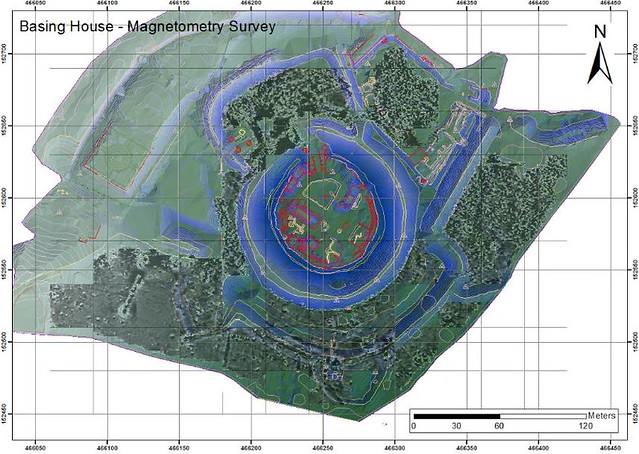
Figure 5 – Magnetometry survey overlain on top of TIN of topographical survey

Another step was to integrate the lidar data procured of the site with GIS and the geophysical survey data as seen in figure 6.

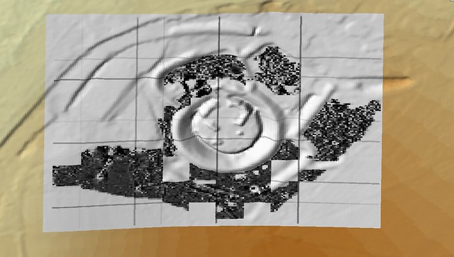
Figure 6 – Geo-physical survey data overlain on top of lidar data of the old house

Lidar data

As we had procured lidar data of the site from the Environment Agency it was decided to experiment on it. A number of features could be seen in the lidar data of the common using a hillshade in ArcMap (or other software). A hillside creates an artificial light source within the software from a set direction and altitude causing shadows to be formed by any raised areas in the lidar data (figure 7); altering the direction and altitude of the light source can reveal different features. More on this can be seen in my blog on processing lidar data.

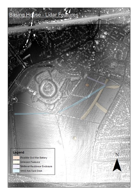
Figure 7 – Lidar data of the Common showing a number of interesting features

Some of these features can also be seen in the geophysical survey of the common undertaken by Clare Allen.

Figure 8 – Geo-physical survey of the common overlain on top of the lidar data

3D visualisation of existing archaeological data

As an aid to understanding the 1960s excavations before we began the 2013 excavations I digitised the plans and sections and created a 3D model in AutoCAD, although far from perfectly accurate the model made it much easier to understanding how features related to each other in this earlier dig and what was missing.

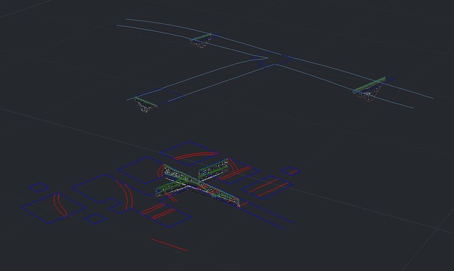
Figure 9 – 3D model created from 1960s excavation data

I experimented with a number of methods of tying the context information from these excavations to the sections, including just displaying it next to the section within AutoCAD.

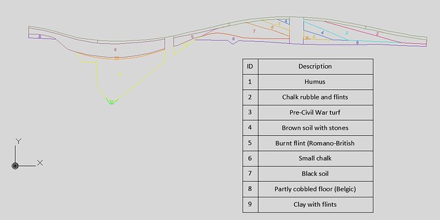
Figure 10 – Digitised section with context information

A later attempt with the data from the 2013 excavations involved the entering of the context information from the excavation into an ARK database (a web accessible database solution created by L-P Archaeology), a hyperlink was created and linked to each context which referenced the relevant webpage associated with the data in the database and this data could then be displayed with one click of the relevant context within AutoCAD.

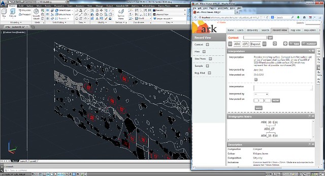
Figure 11 – Digitised section with ARK database record

Special find information could be displayed in the same manner by clicking on the relevant point in the model.

Photogrammetry

Photogrammetry is a technique where 3D models can be created from multiple overlapping photographs by matching the same point in each photograph. As well as using it to record the 2013 excavation I experimented with it to see if slides from the 1978-83 excavations could be used to create a 3D model of this dig. Although it was quite successful much more work needs to be done on the process including surveying in known points on site to aid with stitching the photographs together.

Figure 12 – Photogrammetry model of the old house gatehouse from the 1978-82 excavations

Photogrammetry was also undertaken on box 9A during the 2013 excavations to see how good a 3D model could be created (figure 13), four nails were driven in at the four corners of the box to act as ground control points.

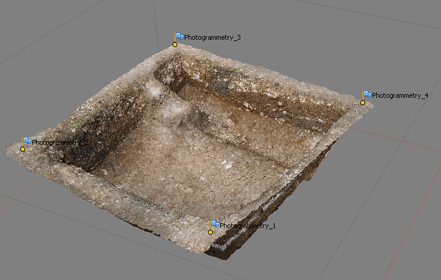
Figure 13 – Photogrammetry model of Box 8A

Figure 13 shows Box 8A with the four ground control points which were surveyed in allowing the integration of the photogrammetry model with ArcMap as can be seen in figure 14 where the model is displayed in its correct position underneath the TIN created from the topographical survey.

Figure 14 – Integration of photogrammetry data with topographical survey within ArcMap

Experimentation was also conducted on recording the excavations from above using a camera attached to a 3m pole (figure 15).

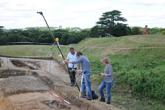
Figure 15 – Elevated photography on a pole being undertaken

This technique allowed the creation of a 3D photogrammetry model of the whole excavation (figure 16).

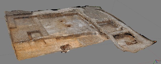
Figure 16 – Photogrammetry model of the 2013 excavations

3D contexts

Due to the fact that the 2013 excavation was recorded with a total station by surveying the outline of contexts and taking levels on the top of them it was possible to experiment with the technique of creating 3D contexts within AutoCAD. First the points from the context were turned into TIN surface (figure 17).

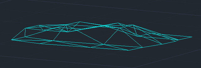
Figure 17 – Wireframe surface created from total station survey of a context

Then the surface was extruded downwards (figure 18)., the same was done with the context below and the second 3D object was subtracted from the first to form a 3D context. This was continued until all the contexts had been created in 3D

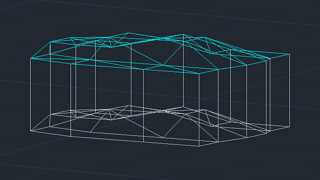
Figure 18 – Wireframe 3D context

Due to the fact that few contexts were actually removed during the excavation part of one of the sections was chosen for this process resulting in the creation of a series of 3D contexts within AutoCAD which could be removed at will virtually recreating the excavation process (figure 19). The volume of the 3D context could also be calculated adding this information to that recorded during the excavation.

Figure 19 – Section of 3D contexts created from total station data

Integration of total station excavation data

Due to the fact that the excavation was recorded digitally using a total station it could easily be incorporated with the topographical survey and building survey data recorded previously. This can be seen in figure 20 where the surfaces created from the excavation data can be seen under the TIN created from the topographical survey in AutoCAD.

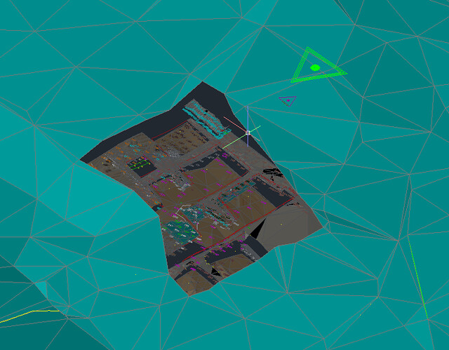
Figure 20 – Integration of excavation data with topographical survey in AutoCAD

While figure 21 shows the point data underneath a TIN surface in ArcMap which is unable to display the surfaces created n AutoCAD.

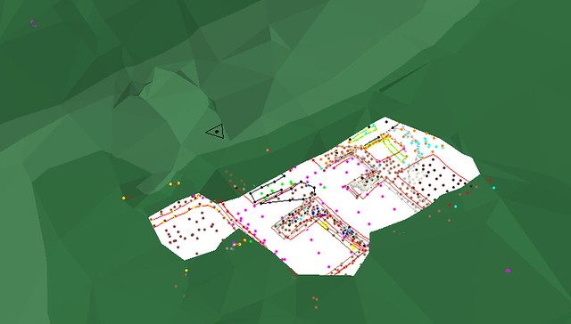
Figure 21 – Integration of excavation data with topographical survey within ArcMap

Conclusions

Although this work demonstrates the potential for the integration of many different types of digital archaeological data a great deal of work still needs to be done to make it a practical process and to solve a number of problems.

–

Blog post by Dan Joyce